Math Review Week 2
Highlights of what I (re)learned in week #2 of my math studies.
L'Hôpital's Rule
If a limit of the form \(\lim_{x \to c} \frac{f(x)}{g(x)}\) yields the indeterminate forms \(\frac{0}{0}\) or \(\frac{\pm\infty}{\pm\infty}\) (and both \(f\) and \(g\) are differentiable near \(c\), with \(g'(x) \neq 0\)), then:
as long as the limit on the right exists (or is \(\pm\infty\)).
For example, if we were trying to evaluate: \(\lim_{x \to 0} \frac{sin(x)}{x}\) we would get \(\frac{0}{0}\), but if we take the derivative of both the numerator and denominator, we can evaluate \(\lim_{x \to 0} \frac{cos(x)}{1} = 1\)
Mean Value Theorem
If \(f\) is continuous on \([a,b]\) and differentiable on \((a,b)\), then there exists some \(c \in (a,b)\) such that
Extreme Value Theorem
If \(f\) is continuous on the closed interval \([a,b]\), then \(f\) attains both an absolute maximum and an absolute minimum on \([a,b]\).
Concavity and Inflection Points
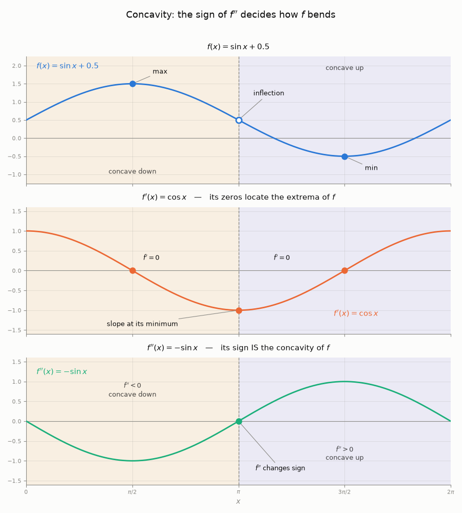
I wanted a nice visualization of concavity with critical points and inflection points. I prompted qwen3.8:27b-mxfp8 (running locally on my laptop) with the following. I then asked for some annotations. It had a bug that took 2 iterations to fix, then I manually enhanced the annotations. An earlier prompt to Claude Opus 5 did a pretty good job in one shot.
Create a new examples/concavity.py file. It should create a plot with 3 charts. The first chart, at the top should plot f(x) = sin(x) + .5 from zero to 2*pi. The second chart, should be of the derivative of f(x). The third chart, at the bottom should be of the 2nd derivative of f(x).
Here is the resulting image:
And here is the code:
# Generated by qwen3.8:27b-mxfp8, then I enhanced most of the annotations manually.

"""Plot f(x), f'(x), and f''(x) to visualize concavity.

f(x)     = sin(x) + 0.5
f'(x)    = cos(x)
f''(x)   = -sin(x)

The third chart drives concavity: where f''> 0 the curve is concave up
("smiling" / a cup that holds water), and where f''< 0 it is concave down
("frowning" / a cup that spills water). Inflection points, where concavity
flips, occur where f''= 0 -- i.e. at x = 0, pi, and 2*pi over this domain.

The first chart marks the max and min and the interior inflection point, and
shades the concave-down (0 < x < pi) vs concave-up (pi < x < 2pi) regions.
The second chart marks the critical points of f' (its local extrema, which lie
where f''= 0). The third chart shades and annotates where f''< 0 and f''> 0
and flags the sign change at x = pi.
"""

import numpy as np
import matplotlib.pyplot as plt


def _annotate(ax, x, y, text, dx, dy, ha="left", va="center"):
    ax.plot([x], [y], "o", color="black", ms=5, zorder=5)
    ax.annotate(
        text,
        xy=(x, y),
        xytext=(x + dx, y + dy),
        ha=ha,
        va=va,
        fontsize=11,
        arrowprops=dict(arrowstyle="->", color="0.3", lw=1.0),
    )


def main() -> None:
    pi = np.pi
    x = np.linspace(0.0, 2.0 * pi, 1000)

    f = np.sin(x) + 0.5
    f1 = np.cos(x)
    f2 = -np.sin(x)

    fig, (ax1, ax2, ax3) = plt.subplots(
        3,
        1,
        sharex=True,
        figsize=(9, 10.5),
        constrained_layout=True,
        gridspec_kw={"height_ratios": [1, 1, 1]},
    )

    # ---- Chart 1: f(x) = sin(x) + 0.5 ----
    ax1.plot(x, f, color="tab:blue", lw=2.0)
    ax1.axhline(0.0, color="0.8", lw=0.8)
    ax1.grid(True, alpha=0.3)
    ax1.set_title(r"$f(x) = \sin(x) + 0.5$", fontsize=13)
    ax1.set_ylabel(r"$f(x)$")
    ax1.set_ylim(-0.95, 1.9)

    # concave down on (0, pi), concave up on (pi, 2pi)
    ax1.axvspan(0.0, pi, color="red", alpha=0.08)
    ax1.axvspan(pi, 2.0 * pi, color="blue", alpha=0.08)
    ax1.text(0.5 * pi, 0.5, "Concave Down", ha="center", va="center", fontsize=12, color="0.0")
    ax1.text(1.5 * pi, 0.5, "Concave Up", ha="center", va="center", fontsize=12, color="0.0")

    _annotate(ax1, 0.5 * pi, 1.5, "max  $(\\frac{\\pi}{2}, 1.5)$", 0.0, -0.3, ha="center", va="top")
    _annotate(
        ax1, 1.5 * pi, -0.5, "min  $(\\frac{3\\pi}{2}, -0.5)$", 0.0, 0.3, ha="center", va="bottom"
    )
    _annotate(ax1, pi, 0.5, "inflection  $(\\pi, 0.5)$", 0.1, 0.5, ha="left", va="bottom")

    # ---- Chart 2: f'(x) = cos(x) ----
    ax2.plot(x, f1, color="tab:orange", lw=2.0)
    ax2.axhline(0.0, color="0.8", lw=0.8)
    ax2.grid(True, alpha=0.3)
    ax2.set_title(r"$f'(x) = \cos(x)$", fontsize=13)
    ax2.set_ylabel(r"$f'(x)$")
    ax2.set_ylim(-1.4, 1.4)

    # critical points of f' are its local extrema (where f''= 0)
    _annotate(
        ax2,
        0.5 * pi,
        0.0,
        "critical:  $f' = 0, at\\ x = \\frac{\\pi}{2}$",
        0.05,
        0.7,
        ha="left",
        va="bottom",
    )
    _annotate(
        ax2,
        1.5 * pi,
        0.0,
        "critical: $f' = 0, at\\ x = \\frac{3\\pi}{2}$",
        -0.1,
        0.2,
        ha="right",
        va="bottom",
    )

    # ---- Chart 3: f''(x) = -sin(x) ----
    ax3.plot(x, f2, color="tab:red", lw=2.0)
    ax3.axhline(0.0, color="0.8", lw=0.8)
    ax3.grid(True, alpha=0.3)
    ax3.set_title(r"$f''(x) = -\sin(x)$", fontsize=13)
    ax3.set_xlabel(r"$x$")
    ax3.set_ylabel(r"$f''(x)$")
    ax3.set_ylim(-1.4, 1.4)

    # shade + annotate where f''<0 (concave down) and f''>0 (concave up)
    ax3.axvspan(0.0, pi, color="red", alpha=0.15)
    ax3.axvspan(pi, 2.0 * pi, color="blue", alpha=0.15)
    ax3.text(
        0.5 * pi, 0.5, "Concave Down\n$f'' < 0$", ha="center", va="center", fontsize=12, color="0.0"
    )
    ax3.text(
        1.5 * pi, -0.5, "Concave Up\n$f'' > 0$", ha="center", va="center", fontsize=12, color="0.0"
    )

    # where f'' changes sign (the inflection point of f)
    _annotate(ax3, pi, 0.0, "$f''$ changes sign\nat $x = \\pi$", -0.2, 0.6, ha="center", va="bottom")

    # ---- shared x-axis ----
    ax1.set_xlim(0.0, 2.0 * pi)
    ax1.set_xticks([0.0, 0.5 * pi, pi, 1.5 * pi, 2.0 * pi])
    ax1.set_xticklabels([r"$0$", r"$\frac{\pi}{2}$", r"$\pi$", r"$\frac{3\pi}{2}$", r"$2\pi$"])

    fig.suptitle(r"Concavity of $f(x) = \sin(x) + 0.5$", fontsize=15)
    plt.show()


if __name__ == "__main__":
    main()
Optimization
A rectangular sheet of cardboard is \(12\) inches by \(20\) inches. Equal-sized squares are cut from each corner, and the sides are folded up to form an open-top box. What size squares should be cut to maximize the volume?
Let \(x\) be the side length of each square cut from the corners. The resulting box has dimensions
Thus, its volume is
Differentiating,
Setting \(V'(x)=0\) gives
Since \(x<6\) is required for a valid box, the maximum occurs at
The maximum volume is therefore
Fundamental Theorem of Calculus — Part 1
If \(f\) is continuous on \([a,b]\), define
Then \(F\) is differentiable on \((a,b)\), and
Fundamental Theorem of Calculus — Part 2
If \(f\) is continuous on \([a,b]\) and \(F\) is any antiderivative of \(f\) on \([a,b]\), meaning
then