Math Review Week 3

Highlights of what I (re)learned in week #3 of my math studies.

Integrating using substitution

Evaluate

\[ \int 2x\cos(x^2)\,dx. \]

Let

\[ u = x^2. \]

Then

\[ du = 2x\,dx. \]

Substituting into the integral gives

\[ \int \cos(u)\,du. \]

Integrating with respect to \(u\),

\[ \sin(u) + C. \]

Finally, substitute \(x^2\) back for \(u\):

\[ \boxed{\sin(x^2) + C}. \]

Integration by parts

Integration by parts is derived from the product rule.

Recall the product rule:

\[ \frac{d}{dx}[f(x)g(x)] = f'(x)g(x)+f(x)g'(x). \]

Let

\[ u=f(x), \qquad v=g(x). \]

Then

\[ du=f'(x)\,dx, \qquad dv=g'(x)\,dx. \]

Multiplying the product rule by \(dx\) gives

\[ d(uv)=v\,du+u\,dv. \]

Rearranging,

\[ u\,dv=d(uv)-v\,du. \]

Integrating both sides,

\[ \int u\,dv = \int d(uv)-\int v\,du. \]

Since

\[ \int d(uv)=uv, \]

we obtain the integration-by-parts formula:

\[ \boxed{\int u\,dv=uv-\int v\,du}. \]

Now let's use it to evaluate an integral.

Evaluate

\[ \int xe^x\,dx. \]

Choose

\[ u=x, \qquad dv=e^x\,dx. \]

Then

\[ du=dx, \qquad v=e^x. \]

Substituting into the integration-by-parts formula,

\[ \begin{aligned} \int xe^x\,dx &=xe^x-\int e^x\,dx\\ &=xe^x-e^x+C. \end{aligned} \]

Therefore,

\[ \boxed{e^x(x-1)+C}. \]

Approximating solutions to differential equations with Euler's method

We can solve ordinary differential equations (ODEs) using Euler's method. For example, let's say y' = y, and y(0) = 1. We'll use a step size of 0.25 to incrementally work through successive steps. At each step, we'll use the current slope to incrementally update y. The smaller the step size, the more accuracy we'll have:

n	tₙ	yₙ	slope f(tₙ, yₙ)	exact y(tₙ) = eᵗⁿ	error
0	0	1.00000	1.00000	1.00000	0.00000
1	0.25	1.25000	1.25000	1.28403	0.03403
2	0.5	1.56250	1.56250	1.64872	0.08622
3	0.75	1.95312	1.95312	2.11700	0.16388
4	1	2.44141	2.44141	2.71828	0.27688
5	1.25	3.05176	3.05176	3.49034	0.43859
6	1.5	3.81470	3.81470	4.48169	0.66699
7	1.75	4.76837	4.76837	5.75460	0.98623
8	2	5.96046	5.96046	7.38906	1.42859

Closed form: (1 + h)^(2/h) = 5.96046

Here is an image to visualize things.

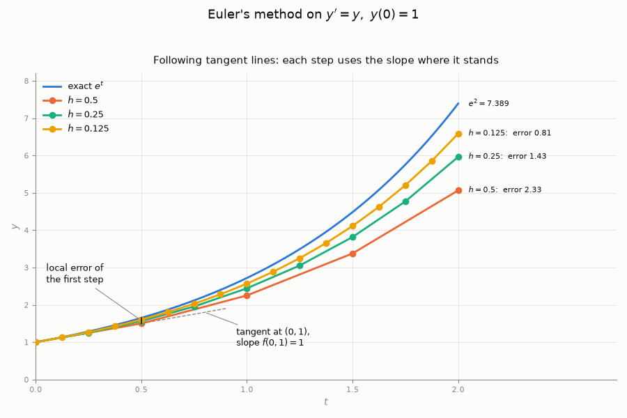
And the Python code to produce the table and image:

# Generated by Claude Opus 5.5

"""Euler's method on y' = y, y(0) = 1 over [0, 2], compared against the exact e^t.

    ODE:     y' = f(t, y) = y          exact solution  y(t) = e^t
    Euler:   y[n+1] = y[n] + h * f(t[n], y[n])

Where the update comes from. The tangent line at (t, y(t)) is the first-order Taylor
step y(t + h) ~ y(t) + h * y'(t). The ODE tells you y'(t) = f(t, y) at any point you
are standing on, so you never need to know the solution in order to take a step. You
evaluate the slope where you are, walk a distance h along that slope, and repeat. The
figure draws exactly that: each polyline is a chain of tangent segments.

Why the error accumulates. Only the first step starts on the true curve. Every later
step evaluates f at a point that is already slightly wrong, so it takes the slope of a
neighboring solution curve rather than the true one. For y' = y the neighboring curves
c * e^t spread apart as t grows, so the early errors are amplified rather than damped.
Every polyline in the figure falls further below e^t the longer it runs. That
happens because e^t is concave up: each tangent segment lies below the curve it touches.

Local error vs global error. One step drops the h^2/2 * y'' term of the Taylor series,
so the LOCAL error per step is O(h^2). Covering [0, 2] takes N = 2/h steps, and N
errors of size O(h^2) add up to a GLOBAL error of O(h). That is what "Euler is a
first-order method" means. Halving h roughly halves the final error, and it also
doubles the work. The errors labeled at t = 2 in the figure show this: going from
h = 1/2 to 1/4 to 1/8 takes the error from about 2.33 to 1.43 to 0.80.

The closed form. For f(t, y) = y the update is y[n+1] = (1 + h) * y[n], so after
N = 2/h steps

    y_N = (1 + h)^(2/h)  ->  e^2   as h -> 0

which is the compound-interest limit: two years at 100% interest, compounded 1/h
times a year. Taking logs gives (2/h) * ln(1 + h) = 2 - h + O(h^2), so
y_N ~ e^2 * e^(-h) ~ e^2 * (1 - h), and for small h the global error is about
e^2 * h. The prediction is not only that the error is O(h); the constant e^2 is
predicted as well.

Usage:

    python euler_method.py
"""

from collections.abc import Callable

import matplotlib.pyplot as plt
import numpy as np

# The same categorical palette used by concavity.py, in fixed slot order. The exact
# solution takes slot 1 (blue), and each Euler run takes the next slot.
BLUE = "#2a78d6"
ORANGE = "#eb6834"
AQUA = "#1baf7a"
YELLOW = "#eda100"
SURFACE = "#fcfcfb"
INK = "#0b0b0b"
MUTED = "#8a8984"

LINEWIDTH = 2.0

T0, Y0, T_END = 0.0, 1.0, 2.0
STEP_SIZES = [(0.5, ORANGE), (0.25, AQUA), (0.125, YELLOW)]


def f(t: float, y: float) -> float:
    """Right-hand side of y' = f(t, y). The t argument is unused here, but it is part
    of the general signature Euler's method works with."""
    return y


def exact(t: np.ndarray) -> np.ndarray:
    return np.exp(t)


def euler(
    f: Callable[[float, float], float], t0: float, y0: float, h: float, n_steps: int
) -> tuple[np.ndarray, np.ndarray]:
    """Take n_steps Euler steps of size h from (t0, y0).

    This is deliberately an explicit loop, because the one line inside it is the whole
    method. Each step depends on the previous one, so there is nothing to vectorize."""
    t = np.empty(n_steps + 1)
    y = np.empty(n_steps + 1)
    t[0], y[0] = t0, y0
    for n in range(n_steps):
        y[n + 1] = y[n] + h * f(t[n], y[n])
        t[n + 1] = t[n] + h
    return t, y


def solve(h: float) -> tuple[np.ndarray, np.ndarray]:
    """Euler on [T0, T_END] with step h. Assumes h divides the interval evenly."""
    return euler(f, T0, Y0, h, round((T_END - T0) / h))


def print_table(h: float) -> None:
    """Print every step for one h as a Markdown table, ready to paste into a post.

    The subscripts are Unicode characters, not t_n, because a pair of underscores in a
    Markdown row would be read as italics."""
    t, y = solve(h)
    print(f"Euler's method for y' = y, y(0) = 1, h = {h}\n")
    print("| n | tₙ | yₙ | slope f(tₙ, yₙ) | exact y(tₙ) = eᵗⁿ | error |")
    print("|--:|--:|--:|--:|--:|--:|")
    for n in range(len(t)):
        print(
            f"| {n} | {t[n]:g} | {y[n]:.5f} | {f(t[n], y[n]):.5f} "
            f"| {exact(t[n]):.5f} | {exact(t[n]) - y[n]:.5f} |"
        )
    print(f"\nClosed form: (1 + h)^(2/h) = {(1 + h) ** (2 / h):.5f}\n")


def style_axes(ax: plt.Axes, title: str) -> None:
    """A recessive grid, recessive spines and ink-colored text, so that nothing
    competes with the data."""
    ax.set_facecolor(SURFACE)
    ax.grid(True, color=MUTED, alpha=0.22, linewidth=0.6)
    for side in ("top", "right"):
        ax.spines[side].set_visible(False)
    for side in ("left", "bottom"):
        ax.spines[side].set_color(MUTED)
    ax.tick_params(colors=MUTED, labelsize=8)
    ax.set_title(title, color=INK, fontsize=11, pad=10)


def plot_solutions(ax: plt.Axes) -> None:
    t_fine = np.linspace(T0, T_END, 400)
    ax.plot(t_fine, exact(t_fine), color=BLUE, linewidth=LINEWIDTH, zorder=3, label="exact $e^t$")

    for h, color in STEP_SIZES:
        t, y = solve(h)
        ax.plot(
            t, y, "o-", color=color, linewidth=LINEWIDTH, markersize=6, zorder=4, label=f"$h = {h}$"
        )
        # The text stays in ink. The legend and the colored endpoint marker already
        # carry identity.
        ax.text(
            T_END + 0.05,
            y[-1],
            f"$h = {h}$:  error {np.e**2 - y[-1]:.2f}",
            color=INK,
            fontsize=8,
            va="center",
        )

    ax.text(T_END + 0.05, np.e**2, f"$e^2 = {np.e**2:.3f}$", color=INK, fontsize=8, va="center")

    # The first h = 0.5 step: walk along the tangent at (0, 1), whose slope is f(0, 1) = 1.
    # The tangent continues dashed past the step to show that it is a straight line.
    # The short vertical bar at t = 0.5 is the local error that this one step introduces.
    t_tan = np.array([0.0, 0.9])
    ax.plot(t_tan, Y0 + f(T0, Y0) * t_tan, "--", color=MUTED, linewidth=1.0, zorder=2)
    ax.plot([0.5, 0.5], [1.5, exact(0.5)], color=INK, linewidth=1.2, zorder=5)
    ax.annotate(
        "tangent at $(0, 1)$,\nslope $f(0, 1) = 1$",
        xy=(0.8, 1.8),
        xytext=(0.95, 0.9),
        color=INK,
        fontsize=9,
        arrowprops=dict(arrowstyle="-", color=MUTED, linewidth=0.8),
    )
    ax.annotate(
        "local error of\nthe first step",
        xy=(0.5, 1.58),
        xytext=(0.05, 2.6),
        color=INK,
        fontsize=9,
        arrowprops=dict(arrowstyle="-", color=MUTED, linewidth=0.8),
    )

    ax.set_xlim(T0, T_END + 0.75)
    ax.set_ylim(0.0, 8.2)
    ax.set_xticks([0.0, 0.5, 1.0, 1.5, 2.0])
    ax.set_xlabel("$t$", color=MUTED, fontsize=10)
    ax.set_ylabel("$y$", color=MUTED, fontsize=10)
    ax.legend(loc="upper left", fontsize=9, frameon=False, labelcolor=INK)
    style_axes(ax, "Following tangent lines: each step uses the slope where it stands")


def build_figure() -> plt.Figure:
    fig, ax = plt.subplots(figsize=(9.0, 6.0), facecolor=SURFACE)
    plot_solutions(ax)
    fig.suptitle(r"Euler's method on $y' = y,\ y(0) = 1$", color=INK, fontsize=13)
    fig.tight_layout(rect=(0.0, 0.0, 1.0, 0.95))
    return fig


def main() -> None:
    print_table(0.25)
    build_figure()
    plt.show()


if __name__ == "__main__":
    main()