Math Review Week 4

Highlights of what I (re)learned in week #4 of my math studies. Shorter week due to traveling.

Solving differential equations by separation of variables

Consider the first-order differential equation

\[ \frac{dy}{dx} = xy \]

The goal is to find a function \(y(x)\) that satisfies this equation.

Step 1: Separate the variables

Divide both sides by \(y\) and multiply both sides by \(dx\):

\[ \frac{1}{y}\,dy = x\,dx \]

Now the left side contains only \(y\), and the right side contains only \(x\). This is called separation of variables.

Step 2: Integrate both sides

Integrate both sides with respect to their respective variables:

\[ \int \frac{1}{y}\,dy = \int x\,dx \]

Evaluating the integrals gives

\[ \ln |y| = \frac{x^2}{2} + C \]

where \(C\) is an arbitrary constant of integration.

Step 3: Solve for \(y\)

Exponentiate both sides to eliminate the logarithm:

\[ e^{\ln |y|} = e^{\frac{x^2}{2}+C} \]

Simplifying,

\[ |y| = e^{x^2/2}e^C \]

Since \(e^C\) is a positive constant, we can absorb the sign and the constant into a new arbitrary constant \(C\). Thus,

\[ y = Ce^{x^2/2} \]

Final answer

The general solution is

\[ \boxed{y(x) = Ce^{x^2/2}} \]

where \(A\) is an arbitrary constant.

Step 4: Verify the solution

Differentiate the proposed solution using the chain rule:

\[ \begin{aligned} \frac{dy}{dx} &= Ce^{x^2/2}\cdot x \\ &= xCe^{x^2/2} \end{aligned} \]

Since \(y = Ce^{x^2/2}\), this becomes

\[ \frac{dy}{dx} = xy \]

which is the original differential equation. Therefore, the solution is correct.

Note: Dividing by \(y\) in Step 1 assumes \(y \ne 0\). The original equation also has the solution \(y=0\), which is included in the general solution by choosing \(A=0\).

Logistic models with differential equations

The logistic growth equation describes a population that grows rapidly at first but slows as it approaches the environment's carrying capacity.

\[ \frac{dN}{dt} = rN\left(1 - \frac{N}{K}\right) \]

where:

• \(N(t)\) is the population at time \(t\).
• \(r\) is the intrinsic growth rate.
• \(K\) is the carrying capacity, or maximum sustainable population.

General solution

Separating variables and integrating yields the logistic function:

\[ N(t) = \frac{K}{1 + Ae^{-rt}} \]

where \(A\) is a constant determined by the initial population.

If \(N(0) = N_0\), then

\[ A = \frac{K-N_0}{N_0} \]

Therefore, the solution with a specified initial population is

\[ \boxed{ N(t) = \frac{K}{1 + \left(\frac{K-N_0}{N_0}\right)e^{-rt}} } \]

Here is an image to visualize logistic growth:

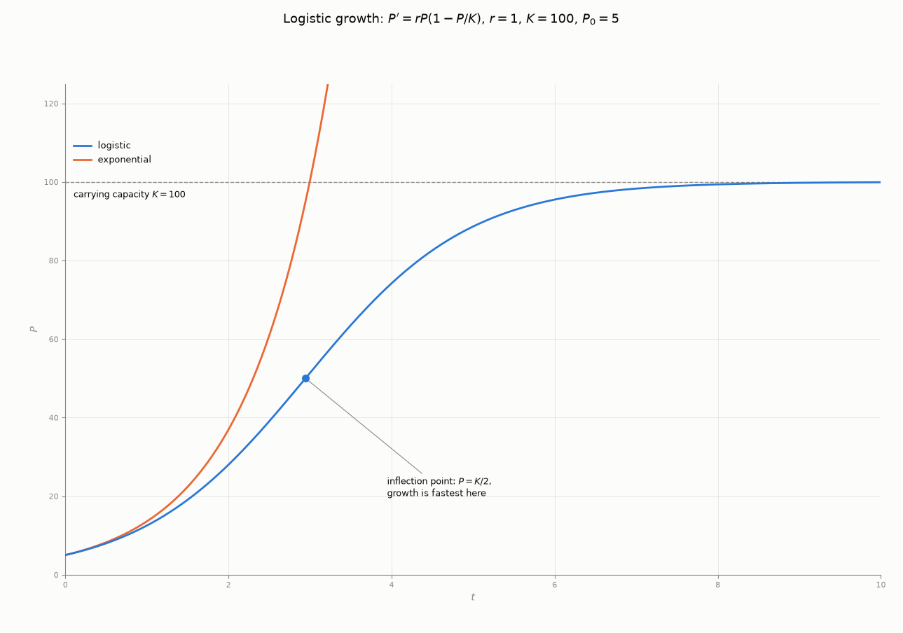
And the Python code that produced it:

# Generated by Claude Sonnet 5.5

"""Logistic growth: P' = r * P * (1 - P/K), compared against unchecked exponential growth.

    Closed form:  P(t) = K / (1 + ((K - P0) / P0) * e^(-r t))

Three things to notice in the figure.

  1. Early on, P is far below K, so (1 - P/K) is near 1 and P' ~ r * P. The logistic
     curve tracks the exponential.
  2. As P approaches the carrying capacity K, the factor (1 - P/K) shrinks toward 0 and
     growth stalls. The curve levels off at K instead of running away.
  3. Growth is fastest at P = K/2, where P * (1 - P/K) is largest. That is the
     inflection point, at t = ln((K - P0) / P0) / r, where the curve switches from
     concave up to concave down.

Usage:

    python logistic_growth.py
"""

import matplotlib.pyplot as plt
import numpy as np

BLUE = "#2a78d6"
ORANGE = "#eb6834"
SURFACE = "#fcfcfb"
INK = "#0b0b0b"
MUTED = "#8a8984"

LINEWIDTH = 2.0

R, K, P0 = 1.0, 100.0, 5.0
T_END = 10.0


def logistic(t: np.ndarray) -> np.ndarray:
    return K / (1 + ((K - P0) / P0) * np.exp(-R * t))


def exponential(t: np.ndarray) -> np.ndarray:
    return P0 * np.exp(R * t)


def build_figure() -> plt.Figure:
    t = np.linspace(0.0, T_END, 400)
    t_inflect = np.log((K - P0) / P0) / R

    fig, ax = plt.subplots(figsize=(9.0, 6.0), facecolor=SURFACE)
    ax.set_facecolor(SURFACE)

    ax.plot(t, logistic(t), color=BLUE, linewidth=LINEWIDTH, zorder=3, label="logistic")
    ax.plot(t, exponential(t), color=ORANGE, linewidth=LINEWIDTH, zorder=2, label="exponential")
    ax.axhline(K, color=MUTED, linestyle="--", linewidth=1.0, zorder=1)
    ax.text(0.1, K - 4, f"carrying capacity $K = {K:g}$", color=INK, fontsize=9)

    ax.plot(t_inflect, K / 2, "o", color=BLUE, markersize=7, zorder=4)
    ax.annotate(
        "inflection point: $P = K/2$,\ngrowth is fastest here",
        xy=(t_inflect, K / 2),
        xytext=(t_inflect + 1.0, K / 2 - 30),
        color=INK,
        fontsize=9,
        arrowprops=dict(arrowstyle="-", color=MUTED, linewidth=0.8),
    )

    ax.set_xlim(0.0, T_END)
    ax.set_ylim(0.0, K * 1.25)
    ax.set_xlabel("$t$", color=MUTED, fontsize=10)
    ax.set_ylabel("$P$", color=MUTED, fontsize=10)
    ax.legend(loc="upper left", bbox_to_anchor=(0.0, 0.9), fontsize=9, frameon=False, labelcolor=INK)

    ax.grid(True, color=MUTED, alpha=0.22, linewidth=0.6)
    for side in ("top", "right"):
        ax.spines[side].set_visible(False)
    for side in ("left", "bottom"):
        ax.spines[side].set_color(MUTED)
    ax.tick_params(colors=MUTED, labelsize=8)

    fig.suptitle(
        rf"Logistic growth: $P' = rP(1 - P/K)$, $r = {R:g}$, $K = {K:g}$, $P_0 = {P0:g}$",
        color=INK,
        fontsize=13,
    )
    fig.tight_layout(rect=(0.0, 0.0, 1.0, 0.95))
    return fig


def main() -> None:
    build_figure()
    plt.show()


if __name__ == "__main__":
    main()